Pandas DataFrames 101
After quite some time since my last post, I like to write today about a topic that I used quite frequently within the last weeks/months: pandas DataFrames.
At some point in your automation story, you need some data for whatever reason from any source that is possible (configuration data, databases etc.). The most basic data that you need every time are connection data for the devices that you like to work with. I know that many people use Excel for this purpose. I like to show you in my next post how to read and work with data from an Excel file in pandas DataFrames. Before we can dive into the Excel topic, I’ll like to show you today the basics how to work with DataFrames in pandas. We’ll take a look how to create a DataFrame from scratch, how to remove and modify data and at the end of the post (and the code example), I show you how to create DataFrames from HTML tables on websites.
The examples for this post is written in a jupyter notebook that is available in my python scripting examples repository on GitHub.
What is pandas?
In a nutshell: Pandas is a library for Data Analysis. The primary target is the work with large data sets and it is therefore build to be very fast and flexible. It’s build on top of numpy, which provides the basic high performance data structures. You can do a lot with these two libraries, but today I show you only some of the basic operations with it.
Both libraries are available via pip for python 2.x and 3.x. You can install it using the following command (numpy is a dependency for pandas):
$ pip install pandasPlease note, that the installation process might take some time depending on your system
Create new DataFrames
A pandas DataFrame is a data structure that represents a table that contains columns and rows. Columns are referenced by labels, the rows are referenced by index values. The following example shows how to create a new DataFrame in jupyter.
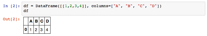
As you can see, jupyter prints a DataFrame in a styled table. You can see that the column values are labeled A, B, C and D and that the rows are index using integers. It is also possible to use different index values (or multiple levels of index values) but this is beyond the scope of this post.
You can access the index and column values using the following attributes:


Lets have a look at some common DataFrame functions that you will need from time to time.
Common Functions in DataFrames
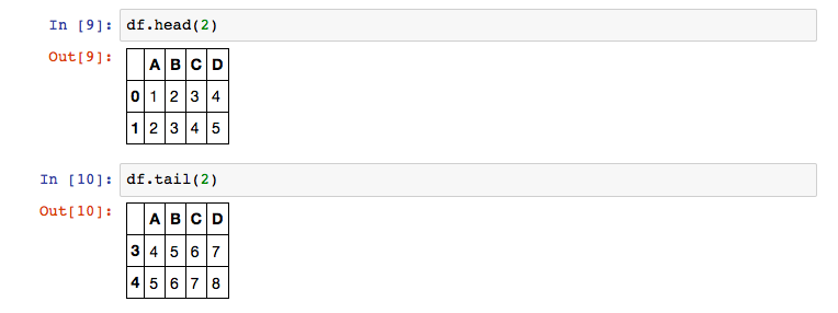
A DataFrame provides a large set of functions, some of them are part of the jupyter notebook. The two functions that I used most times are the head() and tail() function. These functions show only the first (head) or last (tail) elements from a DataFrame.
You find more functions in the workbook, but they are primarily when working with numeric data.
Drop rows from DataFrames
To delete a row from a DataFrame, you need to call the drop() function on your data frame and provide a single index value or a list of index values.
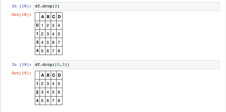
You see that the df.drop(2) statement created new DataFrame that contains all elements except the index value 2. The next drop operation (with index value 0 and 3) contains the index 2 again, because it’s not removed from the original df object.
There are some operations that have an inplace parameter. This prevents the creation of a new slice and performs the operation on the original DataFrame. There are some pitfalls associated to this approach and I recommend to perform the operations that create a copy of the DataFrame.
Select and Edit values
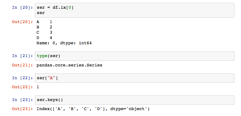
The ix function is used to get a single row. It requires the index value and returns a Series. A Series is a one-dimensional labeled array that comes with the pandas library. You can use a Series like a dictionary to access the values.
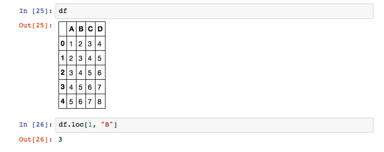
Another way to access the values within a DataFrame is the loc function. This function expects the index and column label of the value that you need.
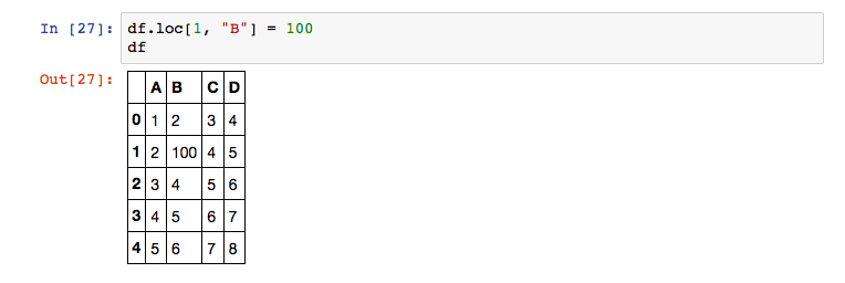
We can also use the loc function to change the value on a specific position.
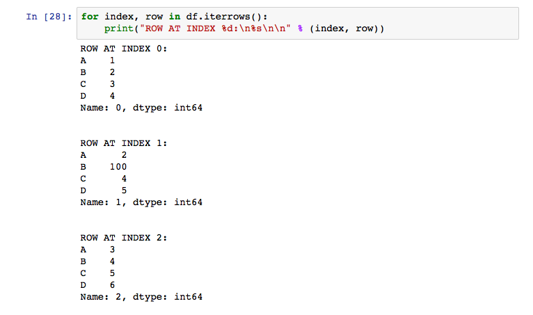
Now we’ve seen how to access values in the DataFrame. To iterate through an entire DataFrame, you need to use the iterrows() function. This function returns the index value and the row as a Series and can be used in the following way:
Filter Values
Iterate through a DataFrame with a lot of elements is not very helpful in many cases. One strength of DataFrames from my perspective are the filtering capabilities. The following example shows a basic filtering example, how to extract all rows from the DataFrame if the A column contains the value 4.
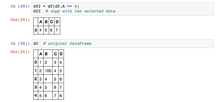
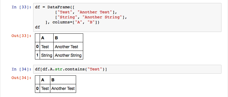
When filtering DataFrames, you need to keep in mind that many operations are not performed on the DataFrame object itself. In most cases, a new slice is created that contains only the data that matches your filtering expression. You can also filter based on text values using the index value of a DataFrame following a str attribute. The following example shows how to filter apply a filter on a DataFrame using text values.
Create DataFrames from other sources
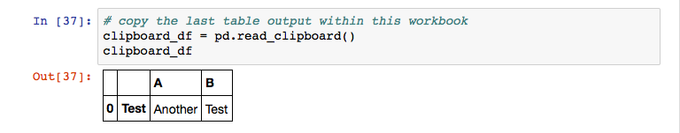
Pandas provides many ways to read data into an DataFrame. This was one of my main reasons to take a deeper look on this library. When using python locally, you can create DataFrames directly from the content of your clipboard. For this reason, pandas provides a read_clipboard() function as you can see in the following example:
I also added an example to the workbook, how to extract tables from a HTML site with the pandas.read_html() function. It requires some additional libraries but it is very useful if you like to extract information from websites.
What’s next?
You can see that DataFrames are a quite useful tool. In my next post, I’ll show you how to work with multiple DataFrames and how to get structured data out of them. Thats it for today, thank you for reading.